출처: https://www.edwith.org/bayesiandeeplearning/lecture/24678?isDesc=false
Probability
학습 목표
Set이 정의되어 있어야 그 위에 Measure를 정의할 수 있고,
Measure가 있어야 Probability를 정의할 수 있습니다.
그래서 이전 학습을 통해 Set과 Measure에 대해서 공부해보았습니다.
이제부터는 베이지안 딥러닝을 공부하기에 앞서 꼭 필요한 개념인 Probability에 대해서 구체적으로 공부해보도록 합시다.
Keywords
- 확률(Probability)
- 표본공간(Sample space)
- 확률 시행(Random experiment)
- 확률 질량 함수(Probability mass function)
- 베이즈정리(Bayes' theorem)
- 기댓값(Expectation)
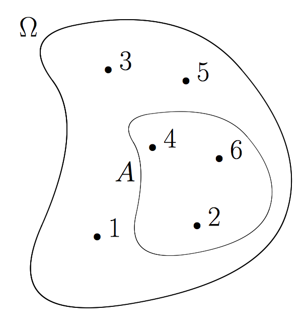
여기서 각각의 눈이 나올 확률은 sample space에서 정의된 면적과 같다.
$$P(\left \{ 1\right \} ) = P(\left \{ 2\right \} ) = P(\left \{ 3\right \} ) = P(\left \{ 4\right \} ) = P(\left \{ 5\right \} ) = P(\left \{ 6\right \} ) = 1/6$$
$$P(A) = P(2, 4, 6) = P(\left \{ 2\right \} ) + P(\left \{ 4\right \} ) + P(\left \{ 6\right \} ) = 1/2$$
- The random experiment should be well defined.
- The outcomes are all the possible results of the random experiment each of which canot be further divided. (outcome $\neq$ sample space)
- The sample point $ w$: a point representing an outcome.
- The sample space $\Omega$
: the set of all the sample points. - Definition (probability)
- $P$ defined on a measurable space $(\Omega, \mathcal{A})$ is a set function
$P$ : $\mathcal{A} \rightarrow [0, 1]$ such that (probability axioms). ($A$는 $\sigma$-field 이며, 0에서 1사이로 measure되고)- $P(\varnothing )=0$ (empty set은 0)
- $P(A) \geq 0 \forall A \subseteq \Omega$ (항상 0이상이고)
- For disjoint sets $A_i$ and $A_j \Rightarrow P(\cup^k_{i=1}A_i)=\sum_{i=1}^{k}P(A_i)$ (countable additivity, disjoint set에 대해서 더하면 더해지는)
- $P(\Omega)=1$ (normalize 되었기 때문에 set 전체가 들어가면 1)
- $P$ defined on a measurable space $(\Omega, \mathcal{A})$ is a set function
- probability allocation function
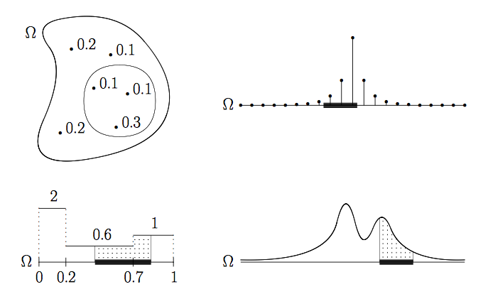
- For discrete $\Omega$: (probability mass function)
$p:\Omega \rightarrow [0,1]$ such that $\sum_{w\in \Omega}p(w)=1$ and $P(A)=\sum_{w\in A}p(w)$ - For continuous $\Omega$: (probability distribution function)
$f:\Omega \rightarrow [0, \infty)$ such that $\int_{w\in \Omega}f(w)dw=1$ and $P(A)=\int_{w\in \Omega}f(w)dw$. - Recall that probability $P$ is a set function $P : A \rightarrow [0; 1]$ where $A$ is a $\sigma$-field.
:결국 sample space에서 확률의 정의를 만족하는 함수들을 찾다보니 gaussian distribution 같은 분포가 나온 것
- For discrete $\Omega$: (probability mass function)
- conditional probability of A given B:
$$P(A|B)\overset{\underset{\mathrm{def}}{}}{=}\frac{P(A\cap B)}{P(B)}$$ - Again, recall that probability P is a set function, i.e., $P : A \rightarrow [0; 1]$.

- From the definition of conditional probability, we can derive:
- chain rule:
$P(A \cap B) = P(A|B)P(B)$
$P(A \cap B \cap C) = P(A|B \cap C)P(B \cap C) = P(A|B \cap C)P(B|C)P(C)$ - total probability law:
$P(A) = P(A \cap B) + P(A \cap B^C ) \\= P(A|B)P(B) + P(A|B^C )P(B^C )$ - Bayes' rule
$p(B|A)=\frac{P(B\cap A)}{P(A)}=\frac{P(A\cap B)}{P(A)}=\frac{P(A|B)P(B)}{P(A)}$ - When B(로또를 맞을 확률) is the event that is considered and A(전날 밤에 꾼 꿈) is an observation,
- $P(B|A)$ is called posterior probability.
- $P(B)$ is called prior probability.
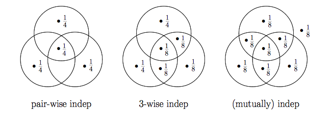
- independent events $A$ and $B$: $P(A \cap B) = P(A)P(B)$

- independent $\neq$ disjoint, mutually exclusive
Random variable
학습 목표
이전 수업을 통해서 확률에 대해서 공부하면서, 확률 공간에 대해서 정의하였습니다.
확률 공간에서는 확률적인 과정에 따라 값이 결정되는 변수가 있는데
그 변수를 확률 변수(Random variable)이라고 부릅니다.
이번 시간에는 확률 변수에 대해서 공부해보도록 해요.
Keywords
- 확률변수(Random variable)
- 확률공간(Probability space)
- 확률 밀도 함수(Probability density function)
- 상관분석(Correlation analysis)
- random variable:
A random variable is a real-valued function defined on $\Omega$ that is measurable w.r.t. the probability space $(\Omega,A,P)$ and the Borel measurable space $(\mathbb{R}, \mathcal{B})$, i.e.,
$X : \Omega \rightarrow \mathbb{R}$ such that $\forall B \in \mathcal{B}, X^{-1}(B)\in A.$
:sample space에서 하나의 원소가 특정 실수에 대응되는 함수, 확률은 sample space $\sigma$-field 에서 정의된 set function
:여기서 inverse image(역함수)로 표시한 것은 주사위의 1과 2가 나올 확률을 구하기 위해 1과 2가 차지하는 면적을 구하기 위해 원래 sample space에서 만들어지는 $\sigma$-field 안에 들어가게하고 싶은 것
*Borel set: 실수들의 집합($\mathbb{R}$)으로 만들어지는 $\sigma$-field
- What is random here?
: sample space에서 하나를 뽑는 것, 함수이기 때문에 그에 해당하는 값이 튀어나옴 - What is the result of carrying out the random experiment?
: 결과는 관측치가 하나 나오는 것
- What is random here?

- Random variables are real numbers of our interest that are associated with the outcomes of a random experiment.
- $X(w)$ for a specific $w\in \Omega$ is called a realization. (즉, sampling이 realization)
- The set of all realizations of $X$ is called the alphabet of $X$. (주사위를 던질 때 alphabet은 1~6)
- We are interested in $P(X \in B)$ for $B \in \mathcal{B}$:
$P(X \in B) \overset{\underset{\mathrm{def}}{}}{=} P(X^{-1}(B)) = P(\left \{w : X(w) \in B \right \})$
:역함수가 차지하는 면적을 계산하는 것이 확률 - discrete random variable: There is a discrete set
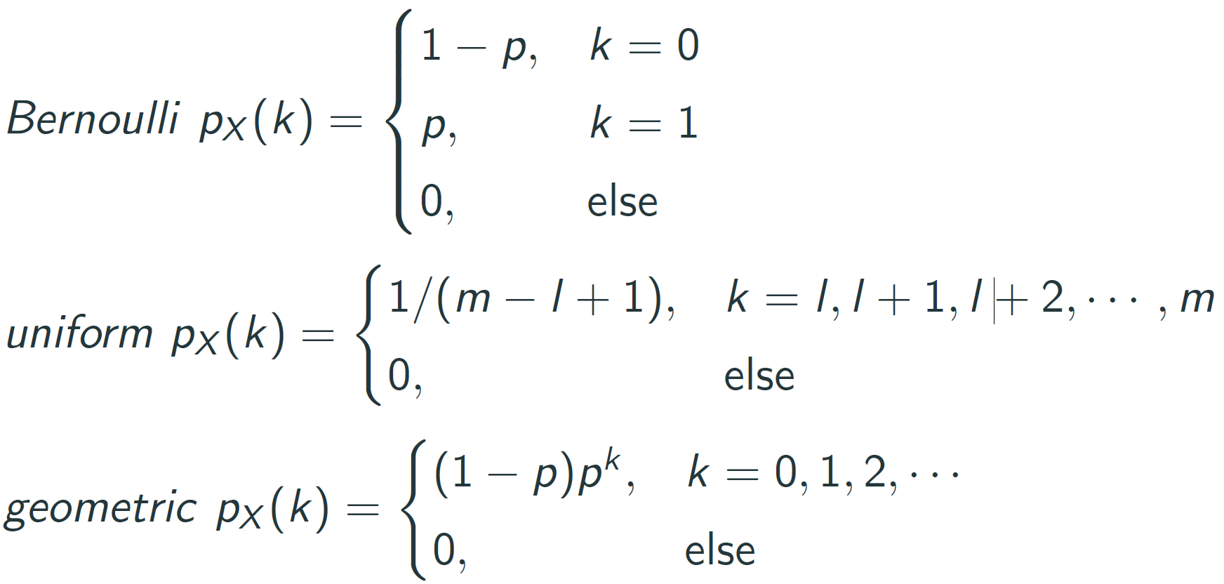
$\left\{ x_i:i=1,2,...\right\}$ such that $\sum P(X=x_i)=1$ (X라는 random variable이 x_i 값이 나올 면적의 크기) - probability mass function: $p_X(x) \overset{\underset{\mathrm{def}}{}}{=}P(X = x)$ that satisfies
- $0\leq p_X(x) \leq 1$
- $\sum_x p_X(x)=1
- $P(X\in B) = \sum_{x\in B}p_X(x)$
- example: three fair-coin tosses
- $X$ = number of heads
- probability mass function (pmf)
$$p_X(x)\left\{\begin{matrix}
1/8, & x=0 \\
3/8, & x=1 \\
3/8, & x=2 \\
1/8, & x=3 \\
0, & \texttt{else} \\
\end{matrix}\right.$$ - $P(X\geq 1)=\frac{3}{8}+\frac{3}{8}+\frac{1}{8}=\frac{7}{8}$
- continuous random variable
There is an integrable function $f_X (x)$ such that
$P(X\in B) =\int _{B}f_X(x)dx$ - probability density function
$f_X(x)\overset{\underset{\mathrm{def}}{}}{=}\texttt{lim}_{\Delta x\rightarrow 0}\frac{P(x< X\leq x+\Delta x)}{\Delta x} $ that satisfies
:pmf와 다른점은 단일 값의 확률은 면적이 0이기 때문에 0이다
- $f_X(x) > 1$ is possible
- $\int_{\infty }^{-\infty } f_X(x)dx=1$
- $P(X\in B)=\int_{x\in B}f_X(x)dx$

$$EX\overset{\underset{\mathrm{def}}{}}{=}\left\{\begin{matrix}
\sum_x xp_X(x), & \texttt{discrete}X \\
\int_{\infty}^{\infty}xf_X(x)dx, & \texttt{continuous}X \\
\end{matrix}\right.$$
- Conditional expectation $E(X|Y)$ (mean 0 gaussian의 expectation 은 0이다. 즉, random variable의 expectation은 radom variable이 아니라 그 평균이다. 그러나 다른 random variable (Y)에 contional하게 되면 그 expectation ($E(X|Y)$)는 random variable이 된다.)
- Expectation $E(X)$ of random variable $X$ is $EX=\int xf_X(x)dx$ and is a deterministic variable.
- $E(X|Y)$ is a function of $Y$ and hence a random variable.
- For each $y$, $E(X|Y)$ is $X$ average over the event where $Y = y$.

- Definition (conditional expectation)
- Given a random variable $Y$ with $\mathbb{E}|Y| < \infty$ defined on a probability space $(\Omega,A,\mathbb{P})$ and some sub-$\sigma$-field $\mathcal{G} \subset \mathcal{A}$ we will define the conditional expectation as the almost surely unique random variable $\mathbb{E}(Y|\mathcal{G})$ which satisfies the following two conditions
- $(Y|\mathcal{G})$ is $\mathcal{G}$-measurable.
- $\mathbb{E}(YZ) = \mathbb{E}(\mathbb{E}(Y|\mathcal{G}Z))$ for all $Z$ which are bounded and $\mathcal{G}$-measurable.
- Conditional expectation $E(X|Y)$ with different $\sigma$-fields.
- Given a random variable $Y$ with $\mathbb{E}|Y| < \infty$ defined on a probability space $(\Omega,A,\mathbb{P})$ and some sub-$\sigma$-field $\mathcal{G} \subset \mathcal{A}$ we will define the conditional expectation as the almost surely unique random variable $\mathbb{E}(Y|\mathcal{G})$ which satisfies the following two conditions

- Moment
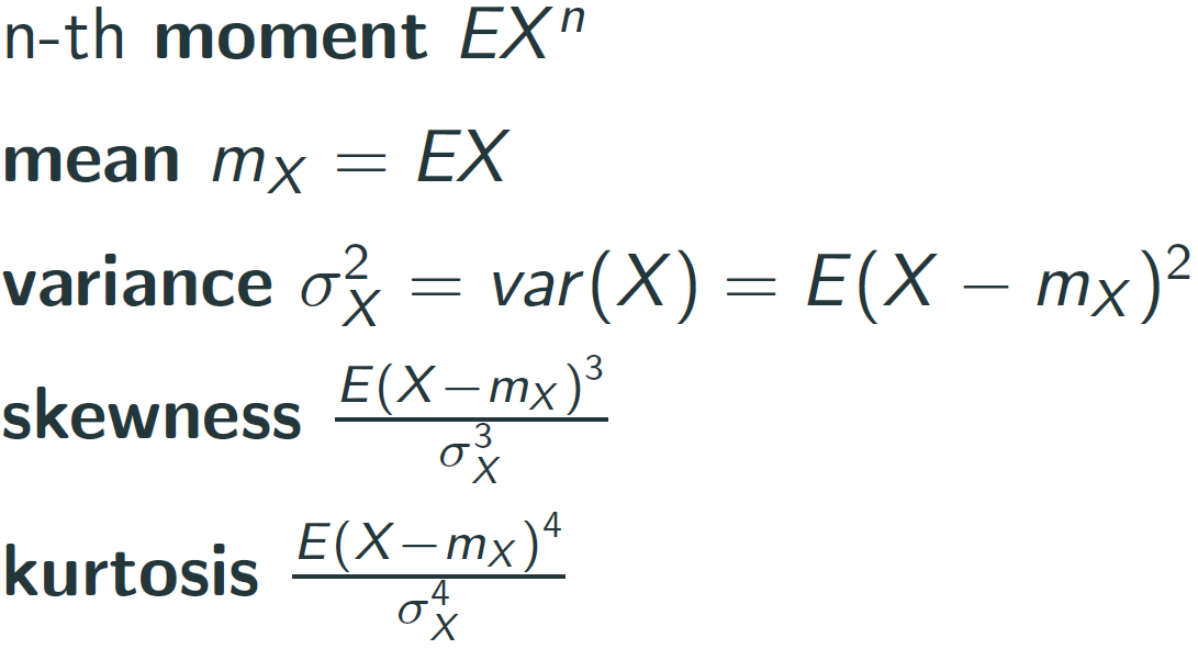
평균은 분포를 고려하지 않기 때문에 다른 분포를 의미하는 다른 수치들과 함께 봐야한다. - Joint Moment

'교육 > Bayesian Deep Learning' 카테고리의 다른 글
| 1-1) Elementary of mathmatics (0) | 2022.11.22 |
|---|
